Showing posts with label networking. Show all posts

Tuesday, July 26, 2011

Network Performance Tools

Links to some of the most useful free open source tools available for network performance testing, debugging, and monitoring. You may already have some of these installed on your system. Some may be available via RPM or the BSD ports library, etc. These links take you to the source/homepage for each tool. All of these run on Linux/Unix, but many of them also have Windows ports.

Connectivity and Path Testing

    You probably already have these:
  • ping / ping6
  • traceroute / traceroute6
  • tracepath / tracepath6
  • Above are in Linux packages iputils and traceroute. Windows comes with ping/ping6, tracert/tracert6, and pathping.
    Additional related tools:
  • synack - a tcp version of ping
  • fping - ping a list of machines, see what is up
  • traceroute - The "NANOG Traceroute". May have features that your traceroute does not, such as mtu discovery.
  • tcptraceroute - good for finding where ports are blocked. Some modern traceroutes can do the same thing (select protocol TCP).
  • Layer Four Traceroute (LFT) - a fairly powerful TCP traceroute
  • Paris Traceroute - features for tracing load balanced paths
  • scamper - a powerful, scriptable, parallel destination traceroute
  • nmap - for finding open/closed/filtered ports
  • mtr - a combined graphical ping/traceroute tool
  • mturoute.exe - a Windows app for finding path mtu

Multicast Tools

TCP/UDP Testing

Internet2's Testing Tools

  • owamp - one way ping
  • bwctl - front end controller to iperf

Packet Capture and Display

  • wireshark - a network sniffer / protocol analyzer (formerly ethereal)
  • tcpdump - raw packet capture (windows version)
  • tcptrace - tcp data and graphs from tcpdump files
  • xplot - essential for viewing tcptrace output (or get the version on the tcptrace website, which includes a windows port link)
  • gnuplot - good for general purpose graphs
  • xgraph - great for quick and simple graphs (old but good)

Utilization, Monitoring, Flows

  • MRTG - Multi Router Traffic Grapher (loved by all)
  • rrdtool - Round Robin Database Tool (MRTG's little brother)
  • Net-SNMP - SNMP library and tools
  • flow-tools - tools for NetFlow data
  • sflowtool - useful in the translation of sflow to pcap
  • ntop - NetFlow/SFlow analysis and web interface
  • Nagios - powerful open source network monitoring

Tools for Advanced Users Only

  • abing - available bandwidth estimation
  • pchar - path characterization
  • pathrate/pathload - available bandwidth and link capacity estimation
  • abget - available bandwidth estimation from web servers
  • netpipe - a Network Protocol Independent Performance Evaluator
  • hping - the swiss army knife of pings
  • drtcp - performance tuning tool for Windows
  • mping - a windowed ping
  • Note that Microsoft has a multicast ping called mping.
  • web100 - Linux kernel mods/tools for performance debugging
    • If you have a web100 kernel, you can use these tools:
    • ndt - Network Diagnostic Tool
    • npad - Network Path and Application Diagnosis

Friday, July 22, 2011

Infrastruktur Jaringan


Memahami Infrastruktur Jaringan Komputer Dalam Organisasi Anda
Suatu infrastruktur jaringan terdiri dari perpaduan banyak technology dan system. Sebagai administrator jaringan anda harus mumpuni dalam menguasai technology-2 terkait agar nantinya infrastruktur jaringan anda bisa dipelihara dengan mudah, di support dengan baik, dan memudahkan dalam troubleshooting jika terjadi suatu masalah baik itu berupa masalah kecil sampai ambruknya system jaringan anda secara global.
Suatu infrastruktur jaringan adalah sekumpulan komponen-2 fisikal dan logical yang memberikan pondasi konektifitas, keamanan, routing, manajemen, access, dan berbagai macam fitur integral jaringan. Misalkan jika jaringan kita terhubung Internet, maka kita akan lebih banyak memakai protocol TCP/IP suite yang merupakan protocol paling banyak dipakai pada jaringan.
Infrastruktur Fisik
Suatu infrastruktur fisik, sesuai dengan namanya – fisik, maka akan banyak berhubungan dengan komponen fisik suatu jaringan (tentunya sesuai dengan design jaringan yang anda buat) seperti:
  • Yang berhubungan dengan masalah perkabelan jaringan, yaitu kabel jaringan yang sesuai dengan topology jaringan yang anda pakai. Misal jika dalam jaringan anda memakai backbone Gigabit Ethernet maka sudah seharusnya anda memakai kabel CAT5e yang bisa mendukung speed Gigabit.
  • semua piranti jaringan seperti :
    • router yang memungkinkan komunikasi antar jaringan local yang berbeda segmen,
    • switches, bridges, yang memungkinkan hosts terhubung ke jaringan
    • Servers yang meliputi seperti server data file, Exchange server, DHCP server untuk layanan IP address, DNS server dan lain-2, dan juga hosts .
  • Infrastruktur fisik bisa termasuk didalamnya technology Ethernet dan standard wireless 802.11a/b/g/n, jaringan telpon umum (PSTN), Asynchronous Transfer Mode (ATM), dan semua metoda komunikasi dan jaringan fisik nya.
Infrastruktur Logical
Infrastrucktur logical dari suatu jaringan komputer bisa merupakan komposisi dari banyak elemen-2 software yang menghubungkan, memanage, dan mengamankan hosts pada jaringan. Infrastruktur logical ini memungkinkan terjadinya komunikasi antar komputer melewati jaringan fisik yang sesuai dengan topology jaringan. Sebagai contoh dari infrastruktur logical ini adalah komponen-2 seperti
  • Domain Name System (DNS), yang merupakan system untuk memberikan resolusi name dari permintaan resolusi name dari clients.
  • Directory services, yang merupakan layanan directory untuk meng-authentikasi dan authorisasi user untuk masuk dan menggunakan resources jaringan.
  • protocol-2 jaringan seperti protocol TCP/IP, protocol jaringan yang sangat popular dan paling banyak dipakai sebagai protocol jaringan dari berbagai platform jaringan baik berplatform windows, Linux, Unix dan lainnya.
  • System keamanan jaringan seperti:
    • jika anda memakai jaringan Windows server, anda mestinya sudah melengkapi dengan system update patch yang dideploy secara automatis kepada semua host dalam jaringan anda seperti WSUS (Windows System Update Services)
    • System keamanan terhadap virus, kalau untuk kepentingan jaringan yang besar anda sudah seharusnya membangun suatu system antivirus corporate edition dimana semua clients akan terhubung ke server ini untuk download signature datanya secara automatis.
    • System keamanan terhadap segala macam ancaman terhadap jaringan anda yang juga terkait dengan infrastruktur fisik anda seperti firewall, pemakaian IPSec pada koneksi remote VPN dan lainnya.
    • Segala macam policy dan guidelines dari corporate tentang pemakaian resource jaringan juga tidak kalah pentingnya. Misal policy tentang pemakaian email dalam company yang tidak (mengurangi) untuk pemakaian pribadi seperti mailing list yang bisa memungkinkan banyak email spam dalam system exchange anda.
  • software client penghubung ke server, dan lain-2.
Setelah terbentuknya jaringan infrastruktur logical ini anda sebagai administrator perlu mempunyai pengetahuan untuk bisa memahami segala aspek technology yang terlibat didalamnya. Seperti anda harus bisa membuat design IP address untuk bisa dimplementasikan berdasarkan jaringan fisik yang ada, bagaimana anda akan memberikan IP address sebagai identitas masing-2 host pada jaringan, dan juga harus bisa melakukan troubleshooting kalau terjadi permasalahan jaringan yang berhubungan dengan konektivitas, addressing, access, security maupun masalah name resolution.
Dan yang lebih penting juga adalah masalah planning anda dalam menghadapi suatu disaster – suatu bencana dalam jaringan anda. Bagaimana anda menyiapkan terjadinya suatu disaster, dan bagaimana anda akan melakukan restorasi kalau disaster itu benar-2 terjadi dan menyebabkan system anda ambruk. Untuk itu anda harus bisa mengantisipasi sejak dini dengan suatu perencanaan terhadap disaster.

LAN Topology


Talking about the Local area network, we should be familiar with the concept of the LAN topology that we use. There are many types of LAN topologies for different types of networks. We should also be familiar between physical topology and logical topology. Physical topology describes the layout of a network media such as copper cable, fiber optic cable, and most popular today is the wireless. While the logical topology is concerned about logical path through the network that data can take from one place to another.
See also Local area network topology in the real world deployed in industry.
The following are basic types of LAN topology:
  • Bus
  • Star
  • Ring
  • Mesh
  • Hybrids
Bus Topology
The first type of LAN topology is the Bus topology which is the first type used in Ethernet network and consists of coaxial cable connected to all the computers on the LAN network. Each computer connected to the coaxial cable through a BNC-style T-connector. The following figure shows typical Bus topology.
Bus topology
All the computer network devices communicate through the same shared bus – so that’s why a bus is also a logical topology. Typically, collision detection (CD) or collision avoidance (CA) algorithms are used in bus topologies to arbitrate network access along with concepts such as “broadcasts” to reach every device on the cable.
Pro:
  • LAN Bus topology is very simple and inexpensive to implement, there is only one main trunk.
Cons:
  • LAN Bus topology requires proper termination on both ends of the bus. Improper termination will cause the network to be malfunction.
  • One single trunk cable becomes a single point of failure, one break, causes all the network impact.
  • Difficult in troubleshooting since you only have one single cable to share for all the computers on the network.
This type of bus LAN topology is not popular today, and it is part of the past and it is difficult today to find any types BNC type LAN adapter at the market.

LAN Star Topology

The second LAN topology is the Star topology. If you run a network cable from each computer to a centralized point such as a Switch, that is a simple concept behind the star topology. The switch handles the repeating or switching the traffic out to the other nodes on the network. The following figure shows the LAN Star topology.
Star topology
Pro:
  • Management is easy through the Switch at the port level. Administration and management can be done remotely by the authorized administrator. See also switch configuration.
  • Any single failure of the port will not impact the whole network. See also network troubleshooting.
  • Installation of the cable in each port will not disrupt LAN services
  • No termination needed like in bus topology.
You should note that nearly every popular network technology today uses a star topology for its physical implementation.
Ring Topology
The third LAN topology is the Ring topology. Compared to bus and star topologies, ring topologies are more complex but they offer some attractive features. Nodes logically communicate in a ring formation, with each node communicating only directly with its upstream and downstream neighbors.
The following figure shows ring topology. Actually Ring topology is physically implemented using star topology.
Ring topology
In a ring topology, access to the network is controlled through a token that is passed from node to node as the arbitration mechanism. Each node takes its turn at claiming the token as the token passes from neighbor to neighbor, and when a node possesses the token, it takes its turn to transmit onto the ring. A data packet is transferred from one node to the next until it reaches its destination node. After the destination node has received the packet, it modifies the packet to acknowledge receipt and passes it on. Eventually, the packet makes it completely around the ring, and the transmitting node receives it and notes that the receipt has been acknowledged. When the transmitting node is finished, it releases the token to its neighbor, and the process repeats.
Ring topology is primary used by the Token-Ring networks.
Pro:
  • No collision detection mechanism is required, so Token ring provides greater overall bandwidth use.
  • Troubleshooting is easy by the fact that each node only knows its upstream and downstream neighbors.
Cons:
  • The firmware required to manage the ring is somewhat complicated and must be on every network card that participates in the ring
  • Expensive to implement and mostly the LANs today use Ethernet technology which dominate the market today.
Mesh Topology
Other LAN topology is a mesh topology which is an interlacing of multiple connections among several nodes. Typically, a mesh is done for one purpose: redundancy. Any serious campus network must incorporate a mesh to achieve the level of redundancy and fault tolerance that businesses demand from their data networks. There are two types of mesh: full and partial.
The following figure is a typical full mesh LAN topology, each devices has connection to each other devices on the network.
Full mesh topology
Pros:
  • Partial meshes are designed to provide redundancy where it is needed
Cons:
  • Except in the smallest network, a full mesh is not very practical
  • The cost of the full mesh implementation is very expensive.

Hybrid Topologies

In large network environment, you can attach Switches one to another to create larger LAN to support more devices. Hybrid topologies combined the above topologies together to form three popular hybrid topologies: tree, hierarchical star, and star-wireless.
Tree Hybrid Topology
The figure below shows combination topology: the star topology combined together with the bus topology.
Hybrid tree topology
Pro:
  • A single computer failure will not bring the entire network to halt.
  • If one hub malfunctions, it disables only the workstations that are attached to it from communicating on the network. The remaining workstations on the other hubs can continue to function normally
Cons:
  • If any problem with the backbone, each groups of the Switches will become segmented into individual Switch.
Hierarchical Star Topology
For large network environment you can configure switches in hierarchical star topology as shown in the following figure.
Hyrarchical Hybrid topology
Pros:
  • Can be used to build large networks.
  • Switches can be configured redundantly to avoid single point of uplink failures
Cons:
  • Size restrictions due to address space and timing issues without introduction of routing technology. See also Layer 3 Switching
Star Wireless
The most recent hybrid topology has arrived with the advent of wireless technology. Wireless LAN technology in its current implementation requires a user to be in the vicinity of a wireless access point attached to the wired network. See also wireless LAN for more detail.
The star topology is necessary to combine the many access points spread across a building to ensure wireless coverage. All the access points collapse back into the main star hub, where server resources would reside on the network. As wireless technologies continue to evolve, so will the topologies that support them.

Mission Critical WAN Connection with Router Redundancy


In a mission critical WAN connection in the organization, router redundancy should be used. There are many integrated firewall and VPN appliances provide dual WAN link for business networks available in the market which can be configured for load balancing or fail-over. In a fail-over system, when the primary connection fails to function the system will fail-over to the backup connection. Many types of routers include two or more WAN ports to let you use fail-over or load balancing.
Building a large network infrastructure for mission critical networks, having router redundancywith redundant WAN connections is an effective method for ensuring network high availability in the event of a core router or primary link failure. Small businesses can deploy any types of multi WAN routers with load balancing and fail-over feature.
In enterprise networks generally they deploy high end routers and switches with the minimum requirement with regards to Router Redundancy as follows:
  • In environments where network high availability (router and link) is required, a router redundancy solution should be deployed.
  • Either VRRP (Virtual Router Redundancy Protocol) or HSRP (Cisco’s Hot Standby Routing Protocol) can be used for router redundancy.
  • Protocols such as client based RIP, Proxy-ARP and IRDP must not be used as a router redundancy solution.
  • Network failover (convergence) time must be less than 10 seconds (5 seconds ideally).
Router redundancy network diagram
Router Redundancy Diagram
Router redundancy is provided by utilizing dual routers running a router redundancy protocol such as VRRP (Virtual Router Redundancy Protocol) or HSRP (Cisco’s Hot Standby Routing Protocol). This should also be used in conjunction with redundant WAN connections. This provides a high available solution which is transparent to user devices.
Many other immature solutions require client agents on the device or generate significant network overhead. Many of these solutions are also slow to converge and often require client reconfiguration. Both VRRP and HSRP can provide transparent high availability solutions that converge in under a few seconds.
Cisco routers currently only support HSRP. HSRP is a Cisco proprietary protocol which has recently been submitted to the IETF (Informational RFC 2281) for review. Consult Cisco Systems for more information on HSRP. VRRP is universal standards protocol defined in RFC 2338.
The following section provides a brief overview of VRRP and HSRP:
HSRP\VRRP requires no client agents, but rather the client utilizes a virtual IP address for its default gateway. The client sends all inter-network data to this virtual router address. An active router takes on the network characteristics of this virtual IP address, whilst a standby router periodically polls the active router to ensure the router is performing its assigned forwarding tasks. See also other Cisco proprietary routing protocol: EIGRP routing protocols which converge very fast and also industrial routing protocols OSPF routing protocols.
HSRP\VRRP is configured such that if the active router fails, the standby router takes over the active roll almost instantaneously. The client continues to successfully forward data via the virtual VRRP/HSRP router without any knowledge of the router failure

If router redundancy is not used then a single router failure will stop all internetwork communications.
For small businesses that demand fail-over or load balancing feature can use the following routers for redundancy requirements:
Cisco RV082 8-port 10/100 VPN Router – Dual WAN
Cisco RV082 is a dual WAN router which includes VPN features and supports load balancing and fail-over feature. The router is equipped with eight fast Ethernet ports (10/100Mbps) for wired connection to the computers with NIC adapter.
Cisco RV082 supports full IPSec VPN capabilities with up to 100 remote connections. For protection against any threats the router includes advanced SPI firewall.
TL-R4299G Dual WAN router for Internet café / businesses
The TP-Link TL-R4299G is a dual WAN router which includes eight gigabit Ethernet LAN ports. The router supports load balancing that selects the lines automatically according to the loads. The router supports IP and Port based Quality of Services to help you provide high performance that demands bandwidth sensitive applications such as video Tele-conference, streaming multimedia and gaming.
FVS336G Dual Wan Gigabit SSL VPN Firewall
The Netgear FVS336G is a dual Wan Gigabit SSL VPN Firewall which supports up to 25 IPSec VPN tunnels and 10 SSL VPN tunnels simultaneously. The router includes two WAN ports to let you configure as the load balancing or fail-over. The router includes four gigabit Ethernet LAN ports with auto-sensing and auto-uplink.
Click here for more details Netgear FVS336G dual WAN gigabit firewall.
Router redundancy is used in a mission critical environment where uninterruptable internet connection is required. There are many routers which supports dual WAN ports for load balancing or fail-over feature available in the market today for small businesses.


Saturday, June 11, 2011

http://psps.perfsonar.net/status/index.html

The perfSONAR-PS Status Collector and Service allows networks to monitor network elements and make available its operational and administrative status information.The perfSONAR-PS Status Collector can collect status information via a number of methods. It can be configured to run a script allowing it to query devices that the service doesn't natively support, or to consult an existing database of status information. The collector can also be configured to obtain status information directly from the switches and routers.

http://psps.perfsonar.net/status/index.html

Friday, June 10, 2011

Buffer Bloat: The calculations

The buffer-bloat blog posts by Jim Gettys[1][2], are very interesting, and relevant for everybody with a broadband connection (especially asymmetric links). They are well written, but also too long and too many posts.

In this blog post, I'll explain what is going on, by showing how you can calculate your own latency issues.

The issue raised by Gettys, is that buffer-bloat (too big buffers on the network path) has fundamentally broken Internet broadband connections [2].
As buffer-bloat can introduce enough latency to cripple your line. Basically killing the possibility of interactive and realtime services, being delivered (e.g. by companies) over your broadband connection.

I'm very happy to see that Gettys is bring this issue up again.
Back in 2005, I discovered the same issues as Gettys. I wrote my masters thesis[3] about the issue, and even created an Open Source "mitigation" solution the ADSL-optimizer[4]. It seems my solution has not gained a wider use.

The major contribution for my side, is to take the ADSL overhead into account when doing QoS packet shaping. (Everything is in mainline, just use/add the TC options "linklayer adsl" and "overhead", if you already have a Linux box doing QoS on your line.)

The issue is that:
A single TCP upload cause a delay of 1.2 seconds (on a 512 Kbit/s ADSL line)
(see thesis[3] page 21).

Lets calculate what is happening, without going into details of why TCP/IP miss-behaves and cause queues to build (details are in my thesis[3]).

Before starting the calculations, here is a beautiful cite by Jim Gettys[1]:
"Large network buffers can be thought of as 'dark buffers', analogous to 'dark matter' in the universe; they are undetectable under many/most circumstances, and you can detect them only by indirect means. Buffers do not cause problems when they are empty. But when they fill they introduce additional latency (and create other problems, possibly very severe) to other traffic sharing the link."

Given the line speed and the delay, we can calculate the buffer size
(this is the bandwidth-delay product). Due to ADSL overhead the
effective bandwidth is actually 454 Kbit/s of the 512 Kbit/s line,
and the measured delay was 1138 ms.
454 Kbit/s * 1138 ms = 64581 bytes
This, corresponds to the TCP window-size. Thus, this is not the maximum buffer-size of the modem. (Use several TCP connection or UDP to find your maximum ping RTT, and calc your buffer size).

Where does the delay come from?!
The delay consists of different components, the important one in our case is the transmission delay (combined with the packets in queue).

The transmission delay of a 1500 bytes (MTU) packet is:
1500 bytes / 454 Kbit/s = 26.34 ms

Thus, the experienced delay is the time it takes to empty the packets in the queue, which is greatly dependend on the line speed.
E.g. 64000 bytes / 454 Kbit/s = 1127 ms.

With a RTT delay of 150 ms, your interactive SSH connection will feel sluggish.
(A side note on ADSL is that; the processing delay in the ADSL modem can get as large as 60 ms, and is caused by the interleaving depth, but its "fortunately" a constant fixed delay on the path)

Increasing the bandwidth, will reduce the latency, but its not the
solution. Besides, ADSL technology is often limited to a 1024 Kbit/s
upstream link.

The Point:
"ISPs SHOULD configure the buffer size based upon the link bandwidth"

I have a feeling that the ISP just configure a default queue size, and tune the queue size based upon max throughput on their largest product.

The line I did my measurements on, I could see delay on 3.3 sec, thus a buffer-bloat size of 187332 bytes (454 Kbit/s * 3300 ms), or 125 packets at 1500 bytes (MTU). Simply crazy!

For more details on formulas and calculation see thesis page 19 to 27.

Links:
[1] Jim Gettys: introducing-the-criminal-mastermind-bufferbloat
[2] Jim Gettys: whose-house-is-of-glasse-must-not-throw-stones-at-another[3] http://www.adsl-optimizer.dk/thesis/
[4] http://www.adsl-optimizer.dk/
[5] http://en.wikipedia.org/wiki/Jim_Gettys

http://netoptimizer.blogspot.com/2010/12/buffer-bloat-calculations.html

Network latency experiments

Recently a series of blog posts by Jim Gettys has started a lot of interesting discussions and research around the Bufferbloat problem. Bufferbloat is the term Gettys’ coined to describe huge packet buffers in network equipment which have been added through ignorance or a misguided attempt to avoid packet loss. These oversized buffers have the affect of greatly increasing latency when the network is under load.
If you’ve ever tried to use an application which requires low latency, such as VoIP or a SSH terminal at the same time as a large data transfer and experienced high latency then you have likely experienced Bufferbloat. What I find really interesting about this problem is that it is so ubiquitous that most people think this is how it is supposed to work.
I’m not going to repeat all of the details of the Bufferbloat problem here (see bufferbloat.net) but note that Bufferbloat occurs at may different places in the network. It is present within network interface device drivers, software interfaces, modems and routers.
For many the first instinct of how to respond to Bufferbloat is add traffic classification, which is often referred to simply as QoS. While this can also be a useful tool on top of the real solution it does not solve the problem. The only way to solve Bufferbloat is a combination of properly sizing the buffers and Active Queue Management (AQM).
As it turns out I’ve been mitigating the effects of Bufferbloat (to great benefit) on my home Internet connection for some time. This has been accomplished through traffic shaping, traffic classification and using sane queue lengths with Linux’s queuing disciplines. I confess to not understanding, until the recent activity, that interface queues and driver internal queues are also a big part of the latency problem. I’ve since updated my network configuration to take this into account.
In the remainder of this post I will show the effects that a few different queuing configurations have on network latency. The results will be presented using a little utility I developed called Ping-exp. The name is a bit lame but Ping-exp has made it a lot easier for me to compare the results of different network traffic configurations.

My Home Network

The figure below outlines what my home network looks like. It’s pretty standard except for the addition of the Linux server (Dest2) which lives at my local ISP. By tunneling traffic between Dest2 and my home router I can control the downstream traffic in a way not available to most Internet users.
Home network diagram
My Internet connection is PPPoE based and a operates at a the modest speed of ~4Mbps download and ~768Kbps upload.

Experimental Design

In each of the experiments below Ping-exp was run on both hosts A and B, pinging both Dest1 and Dest2, five times per second, with a total of 400 pings (80 seconds).
./ping-exp.py -w test.data -t 'dest1,<IP1>,0' -t 'dest2,<IP2>,0' -i .2 -c 400
[Replace <IP1> and <IP2> if cutting and pasting the above]
In the results below I only show data from HostA because the results are very similar on HostB. I had originally planned to perform some experiments which involved per-host fairness but that will have to wait for another time.
Each network configuration was tested under the four network load scenarios outlined in the table below. In each case there was a short interval of approximately one minute between starting the load and running Ping-exp. All load was generated from HostA.
Load Description
Empty No traffic
Upload 2 TCP uploads to C
Download 3 TCP downloads from C
Both 2 TCP uploads to C and 3 TCP downloads from C

Experiment 1: Defaults

In this experiment all device queues and traffic management configurations were unmodified from the Linux defaults.

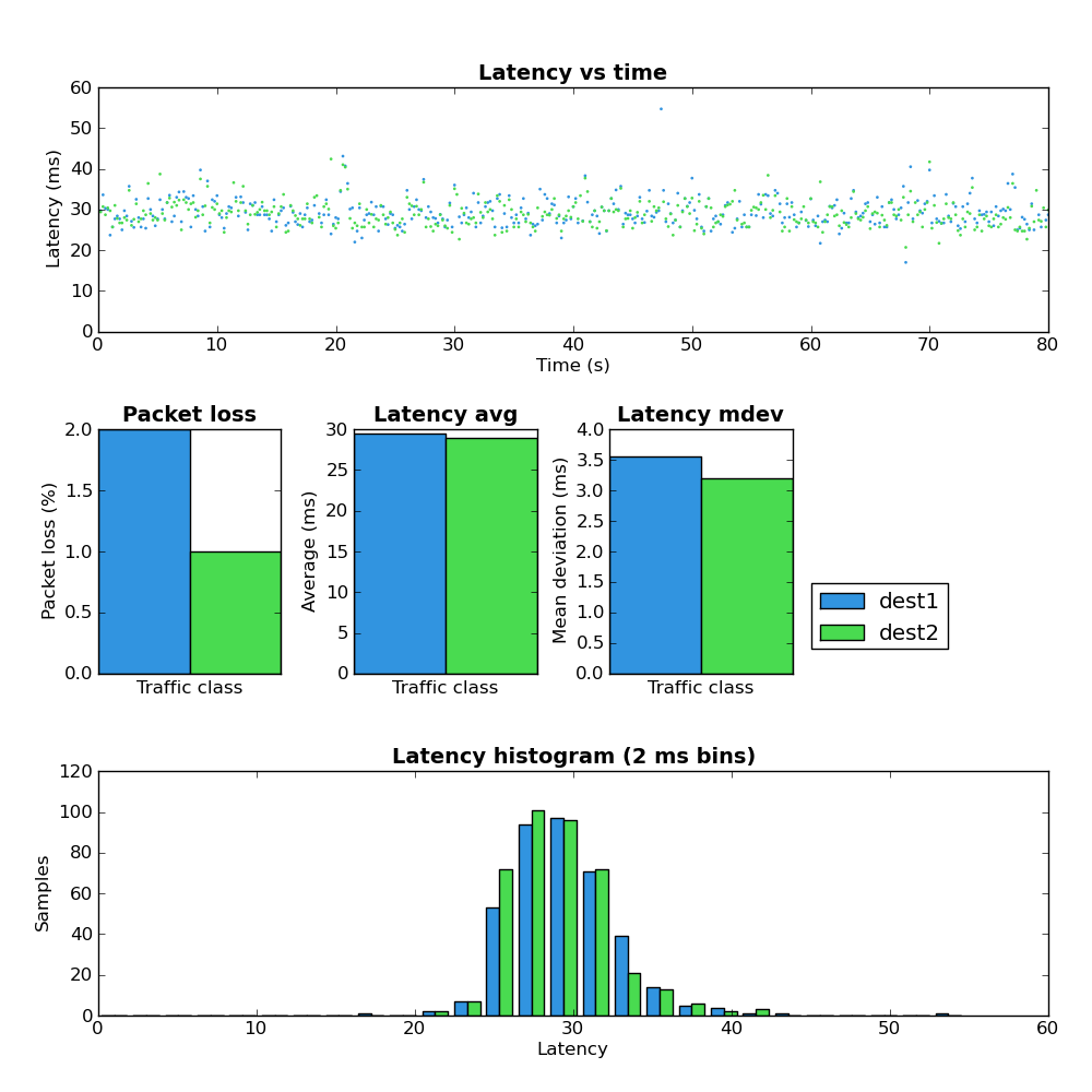
Network Load: Empty

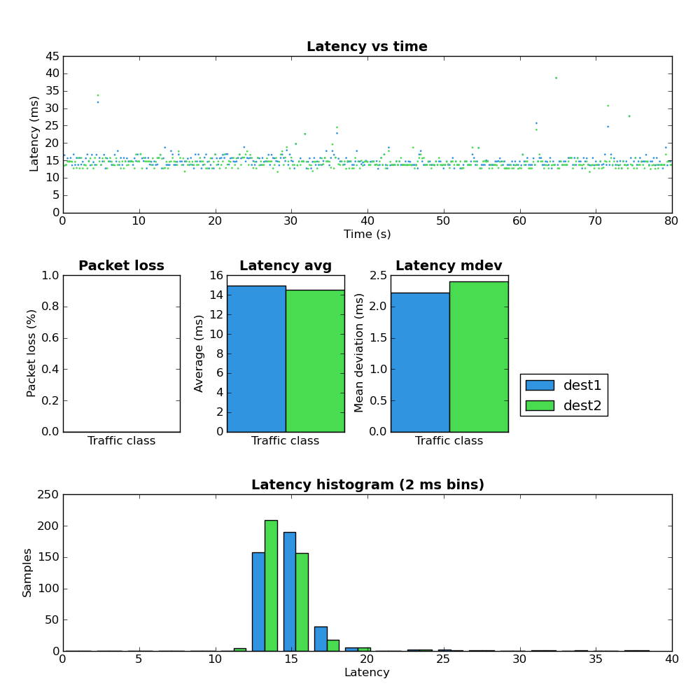
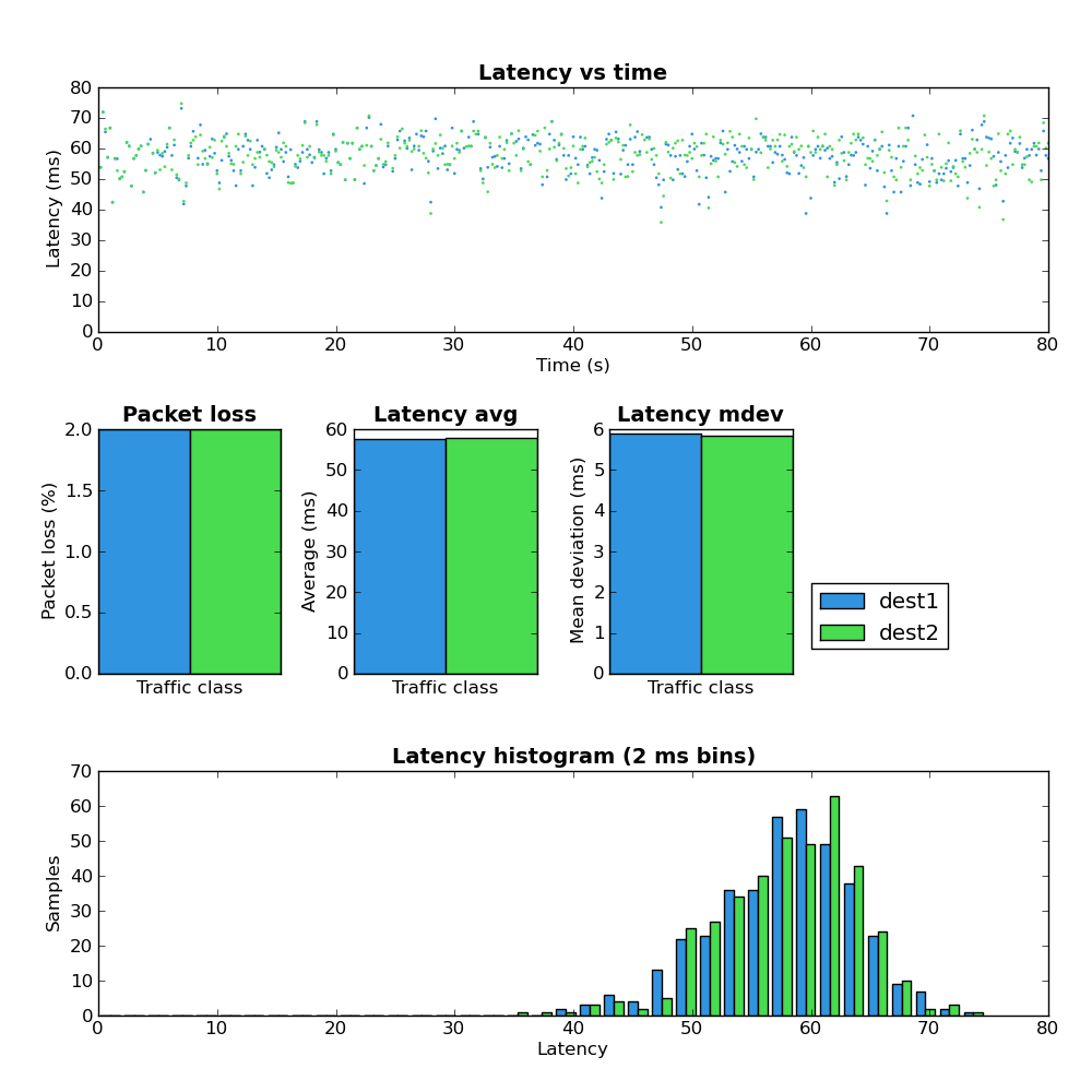
Figure 1: Host A - defaults - empty
Figure 1 provides a baseline for the network with no traffic.

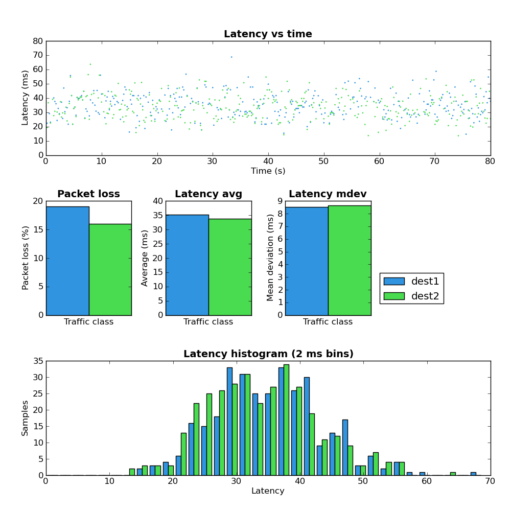
Network Load: Upload

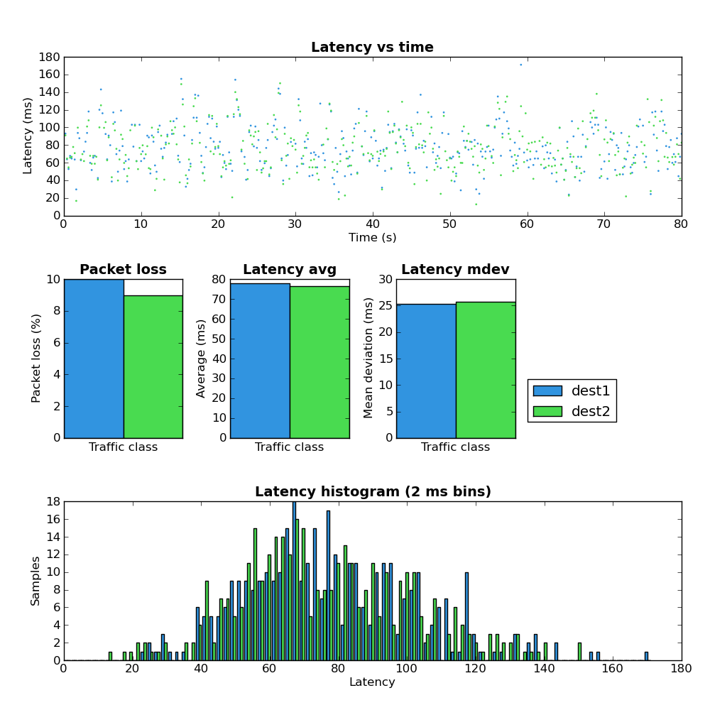
Figure 2: Host A - defaults - upload
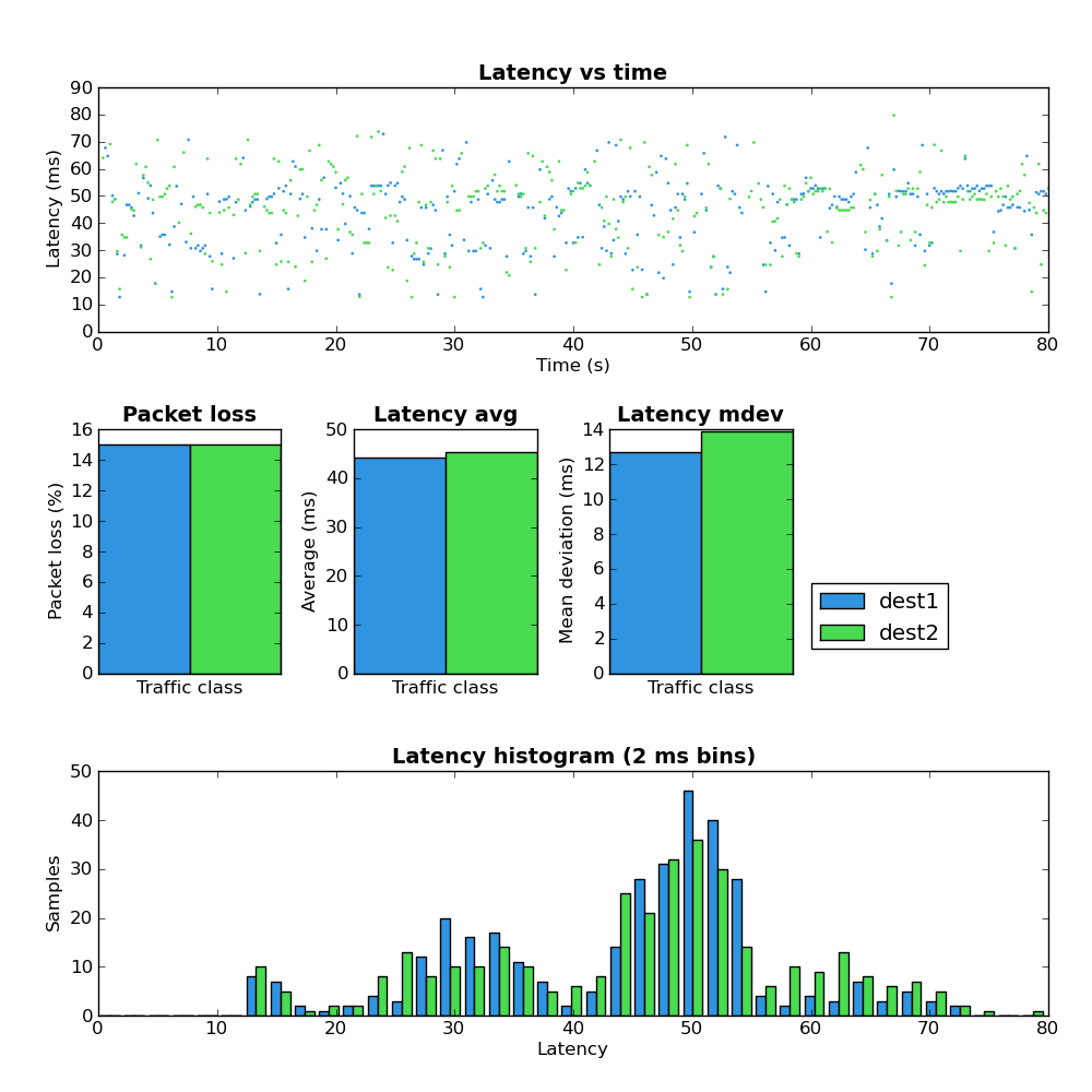
Comparing figure 1 and figure 2 shows that when the upload portion of the link is under load both the latency and jitter greatly increase. However the maximum observed RTT at ~180ms isn’t terribly high which seems to indicate the upstream portion of the network does not suffer from extream Bufferbloat. Notice that the amount of packet loss increased from 0% to ~10%.
Even with the sane maximum latency as mentioned above this amount of packet loss would likely make any interactive service which relies on TCP (such as an SSH terminal) unusable due to the time required to recover from lost packets. I suspect 10% packet would also make VoIP conversations unusable but I don’t have any data to back that up.

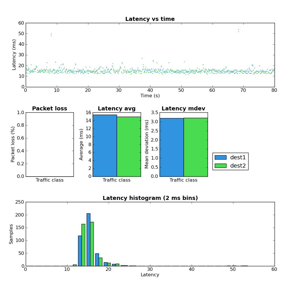
Network Load: Download

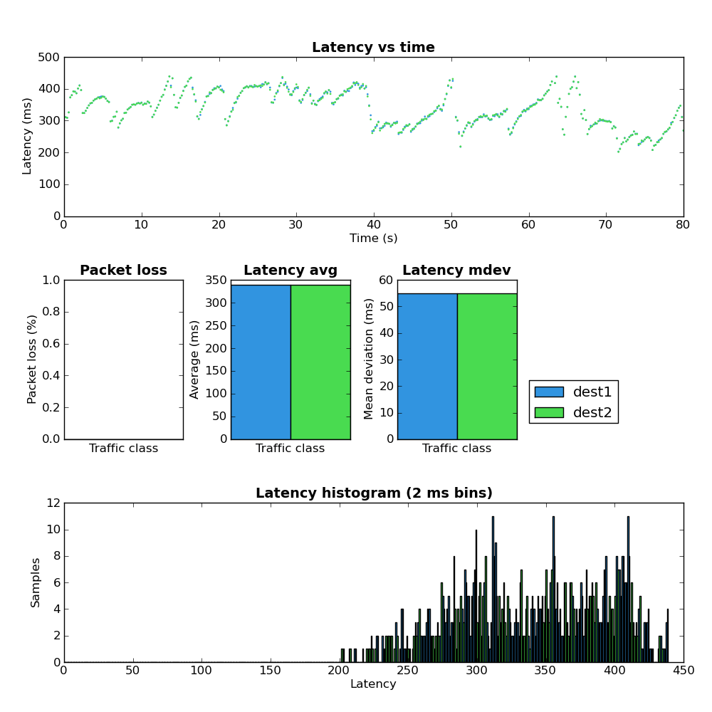
Figure 3: Host A - defaults - download
It’s hard to look at Figure 3 and not immediately be drawn to the interesting latency pattern in the top chart. I suspect that the relatively slow latency increases followed by a sudden latency drop are the result of the network queues filling and then quickly emptying after TCP reduces the send rate when it finally receives a loss event. There are two other things to note in Figure 3:
  • The overall latency is much worse in the download path.
  • There is no packet loss experienced by the test flows.
I’m at a loss to explain the latter point.

Network Load: Both

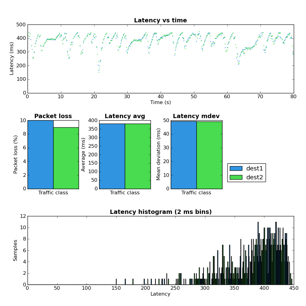
Figure 4: Host A - defaults - both
Figure 4 shows the latency results when under both upload and download load. Here the average latency increases beyond either the upload or download only case and the ‘latency sawtooth’ identified in Figure 3 becomes even more pronounced. The packet loss in Figure 4 is very close to the upload case (Figure 2) which matches well with the download results (Figure 3) where no packet loss was observed.

Experiment 2: Reduce buffers and shape

In this experiment the buffers on both ends of the Internet connection were reduced as follows:
  • Gateway
    • The TX queue length (ifconfig txqueuelen) was reduced to 1 packet for the ppp0 interface as well as the underlying eth2 interface.
    • The queueing discipline on eth2 was changed to a PFIFO with a buffer size of a single packet.
    • The queueing discipline on the ppp0 interface was changed to a PFIFO with buffer size of 3 packets which is equal to approximately 50ms at the maximum link rate.
  • Dest2
    • The TX queue length of the eth0 interface was reduced from the default of 1000 to 10.
    • The queueing discipline on the interface towards the home network was set as a PFIFO with a buffer size of 18 packets which is equal to approximately 50ms at the maximum link rate.
In addition to the above buffer changes, traffic shapers were also added to each end of the IPIP tunnel and set to a value below the available network throughput. This removes the effects of any buffering in intermediate network elements.

Network Load: Empty

As expected performing the test with no network load obtains results very similar to Figure 1.

Network Load: Upload

Figure 5: Host A - low buffers - upload
Comparing Figure 5 with Figure 2 shows a much better latency and jitter profile but the amount of packet loss is somewhat higher (~9%->14%).

Network Load: Download

Figure 6: Host A - low buffers - download
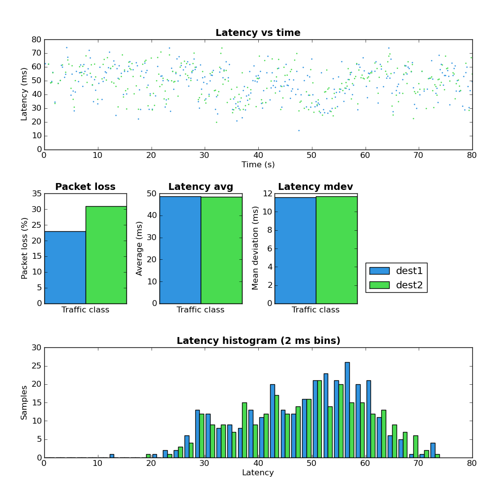
Figure 6 shows no sign of the latency sawtooth behavior observed in Figure 3. This appears to confirm the theory that the large buffers were the cause of this phenomenon. Also note that latency and jitter are vastly improved but there is slightly higher packet loss (0%->2%).

Network load: Both

Figure 7: Host A - low buffers - both
Figure 7 shows a much better latency profile when compared with Figure 4 but note that the packet loss has increased to a very high level.

Experiment #3: Reduce interface buffers and shape plus SFB

Stochastic Fair Blue is an active queue management (AQM) scheme which has been suggested as a possible solution to the buffer bloat problem. Due to the fact that SFB currently requires a custom kernel module I chose not to install it on Dest2. This server isn’t easy for me to get access to should something go wrong. I did however install it on the local gateway to obtain upload results.
The only change between this experiment (#3) and #2 is the replacement of the PFIFO queue on the gateway with a SFB queue. SFB has the ability to mark IP packets via ECN when they experience congestion. Both Host A and Dest2 have ECN enabled and ECN marked IP and TCP packets were observed during this test.
Figure 8: Host A - low buffers - sfb - upload
Comparing figure 8 against figures 2 and 5 shows that SFB does have a better latency profile vs a simple FIFO but the packet loss is also significantly higher. I haven’t done enough experimentation with SFB to really understand how to use it effectively but these results do seem to indicate that it’s worth spending more time with.

Experiment #4: Sane buffers plus SFQ

This experiment maintains the buffer size optimizations from experiments 2 and 3 but adds a SFQ queue to each end of the connection. SFQ aims to create per-flow fairness. On the downstream the SFQ queue length (limit parameter) was set to eighteen and on the upstream it was set to three. Both of these values result in approximately 50ms transmission time.

Network load: Upload

Figure 9: Host A - low buffers - sfq - upload
Figure 9′s direct comparisons are figures 2, 5, 8. Only the SFB case (Figure 8) has lower average latency and all other scenarios have far higher packet loss.

Network load: Download

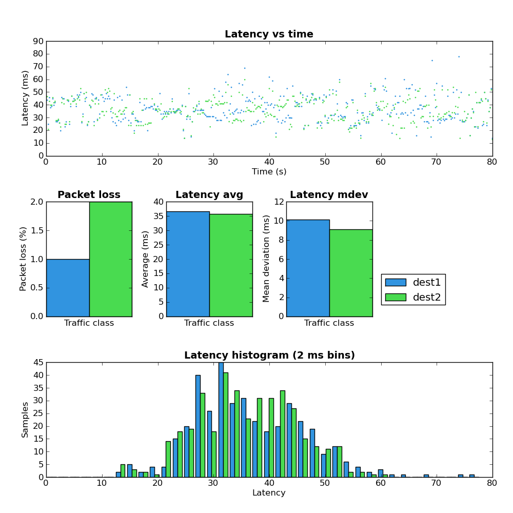
Figure 10: Host A - low buffers - sfq - download
Figure 10′s comparisons are Figures 3 and 6. Figure 10 shows a better latency profile vs the other scenarios with equivalent or better packet loss.

Network load: Both

Figure 11: Host A - low buffers - sfq - both
Comparisons: Figures 4 and 7.
In this test the bidirectionally loaded link shows a lot of packet loss but latency is better than the other scenarios.

Throughput

During these experiments I did not make any effort to compare the overall network throughput. This would be a worthwhile endeavour but anecdotally at least any throughput difference is relatively minor and is a cost worth paying in order to achieve improved latency.

Summary

These experiments show the dramatic difference in network latency which can be obtained by modifying the size of packet buffers and adding a bit of traffic classification (SFQ). Among the tested scenarios, SFQ + sane buffers sizes gives the best performance.
When I started this post I had hoped to go through a few more scenarios but that will have to wait for another time. Specifically I wanted to show the results of the somewhat more complicated scheme that I use on a daily basis. This scheme gives much better results than any of the ones presented above. If you are interested and understand how to use tc you can see the scripts here.

http://www.coverfire.com/archives/2011/02/21/network-latency-experiments/